在 上一节 中我们简单介绍了关联分析的基本知识，规则挖掘任务的定义以及简单说明了剪枝的原理。

现在本节将主要讲解规则挖掘的两个子任务的第一个任务：频繁项集的产生。

首先我们先来看一下在计算过程中候选的频繁项集该如何保存在内存中，也就是我们使用什么样的数据结构对频繁项集进行记录和保存。

格结构 ( lattice structure ) 是我们常用的，用于枚举所有可能的项集的结构。

项集格

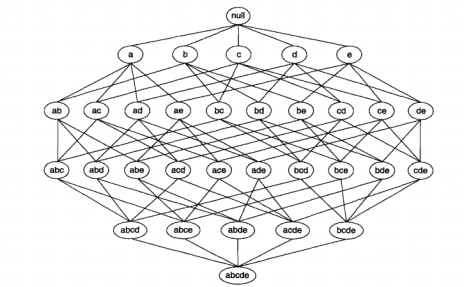
一般来说一个包含 $k$ 个项的数据集可能产生不包括空集在内的 $2^k-1$ 个频繁项集。发现频繁项集的一种暴力方法就是确定格结构中每个候选项集的支持度计数。那么可以得出这种方法需要的开销为将每个候选项集与每个事务进行比较，即进行 $O ( NM \omega )$ 次比较，其中 $N$ 是事务数，$M=2^k-1$ 是候选项集，而 $\omega$ 是事务的最大宽度。

那么如何降低该代价呢？ 降低频繁项集计算复杂度有 3 种主要的方法：

1. 减少候选项集的数目 ( $M$ ) 。下面介绍的先验原理就是一种不用计算支持度而减少某些候选项的有效方法。
2. 减少比较次数。使用更高级的数据结构来存储候选项集或者压缩数据集，以此来减少比较次数。
3. 减少事务数目 ( $N$ ) 。随着候选集的规模越来越大，能支持项集的事务将会越来越少。

先验原理

该方法可实现使用支持度度量来减少频繁项集产生时需要探查的候选项集个数。

先验原理

如果一个项集是频繁的，则它的所有子集一定也是频繁的。

相反，如果项集 {a, b} 是非频繁的，那么它的所有超集一定是也非频繁的，那么整个包含 {a, b} 超集的子图也可以被立即剪枝。这种基于支持度度量修剪指数搜索空间的策略被称为 基于支持度的剪枝 ( support-based purning )。这种剪枝策略依赖于支持度度量的一个关键性质，即一个项集的支持度绝不会超过它的子集的支持度。这个性质也被称为支持度度量的 反单调性。

反单调性

如果对于项集 $Y$ 的每个真子集 $X$( 即 $X \subset Y$ ) ，有 $f ( Y ) \le f ( X )$，那么度量 $f$ 具有反单调性。

Apriori 算法的频繁项集产生

Apriori 算法是第一个关联规则挖掘算法，它开创性地使用基于支持度的剪枝技术，系统地控制候选项集的指数增长。

我们以下表为例，看一下 Apriori 是如何操作的：

设定阈值支持度为 60%，即最小支持度为 3。

TID	面包	牛奶	尿布	啤酒	鸡蛋	可乐
1	1	1	0	0	0	0
2	1	0	1	1	1	0
3	0	1	1	1	0	1
4	1	1	1	1	0	0
4	1	1	1	0	0	1

表 2.1

1. 找出所有的 1-项集并计算其支持度。

   项	计数
   {啤酒、}	3
   {面包、}	4
   {可乐、}	2
   {尿布、}	4
   {牛奶、}	4
   {鸡蛋、}	1

2. 将低于支持度阈值的项丢弃，剩下频繁的项。

   项	计数
   {啤酒、}	3
   {面包、}	4
   {尿布、}	4
   {牛奶、}	4

3. 用剩下的频繁项生成 2-项集。

   项	计数
   {啤酒， 面包、}	2
   {啤酒， 尿布、}	3
   {啤酒， 牛奶、}	2
   {面包， 尿布、}	3
   {面包， 牛奶、}	3
   {尿布， 牛奶、}	3

4. 重复步骤 2，用频繁项生成 3-项集。

   项	计数
   {面包， 尿布， 牛奶、}	2

我们可以看到，使用先验原理之后，候选项集相较于暴力算法减少了 68%。

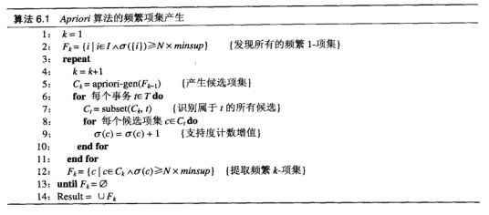
下面给出书中的伪代码

Apriori pseudocode

候选项集的产生与剪枝

上面的伪代码中有两个非常重要的函数：candidate-gen 和 candidate-prune。这两个函数分别完成如下两个操作产生候选项集和剪枝非必要项。

1. 候选项集的产生。 该操作由前一次迭代发现的频繁 ( k-1 ) -项集产生新的候选 k-项集。
2. 候选项集的剪枝。 该操作基于支持度的剪枝策略，删除一些候选 k-项集。

注意

完成这种剪枝并不需要计算这些 k-项集的实际支持度 ( 支持度可以通过将这些项集和每个事务进行比较获得 ) 。

候选项集的产生

有效的候选产生过程必须是 完全 且 无冗余 的。完备的 是指如果候选集产生过程中未遗漏任何频繁项集，无冗余 是指候选项集产生过程中对同一候选项集的产生不超过两次。

接下来介绍几种候选项集的产生过程。

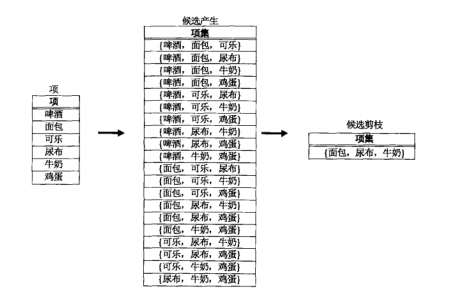
暴力方法

把所有的 k-项集都看作可能的候选，然后使用剪枝去除不必要的候选项。假设 $d$ 为项的总数，第 $k$ 层的候选项集的数目为 $C_d^k$。

该方法的优点是算法简单，缺点是需要考察的项集数量很大，所以候选剪枝的开销也特别大。

暴力方法

$F_{k-1} \times F_{1}$ 方法

用 1-项集的频繁项来扩展每个频繁 ( k-1 ) -项集。

$F_{k-1} \times F_{1}$ 方法

从图中可以看出相较于暴力方法获得的 $C_6^3 = 20$ 个项集，该方法只产生了 4 个项集，数量大大减少。但是该方法仍会产生大量不必要的候选。

注意

以上提到的方法都很难避免重复产生候选项集。例如，{面包， 尿布， 牛奶} 可以通过合并项集 {面包， 尿布} 和 {牛奶} 产生，而且还可以通过 {面包， 牛奶} 和 {尿布} 合并产生，或者合并 {尿布， 牛奶} 和 {面包} 产生。

避免重复产生候选项集的一种方式是使用字典序，确保每个频繁项集中的项以字典序存储。然后每个 ( k-1 ) -项集 $X$ 只用字典序比 $X$ 中所有的项都大的频繁项进行扩展。

如果协同 $F_{k-1} \times F_{1}$ 方法和字典序则仅仅会产生 2 个候选 3-项集。因为 {啤酒， 面包} 不是频繁 2-项集，所以 {啤酒， 面包， 尿布} 和 {啤酒， 面包， 牛奶} 不会产生。

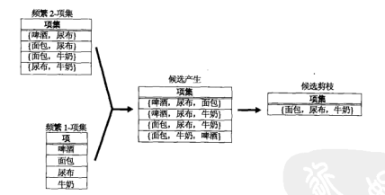
$F_{k-1} \times F_{k-1}$ 方法

这个方法也是 Apriori 算法中 candidate-gen 函数使用的方法。

将一对频繁 ( k-1 ) -项集进行合并，仅当其前 k-2 个项按照字典序都相同。令 $A = \{a_1, a_2, \dots, a_{k-1}\}$ 和 $B = \{b_1, b_2, \dots , b_{k-1}\}$ 是一对符合字典序的频繁 ( k-1 ) -项集，合并 $A$ 和 $B$，如果它们满足如下条件：

$$\tag{2.1} a_i \times b_i ( i=1,2,\dots, k-2 ) \quad AND \quad a_{k-1} \neq b_{k-1}$$

$F_{k-1} \times F_{k-1}$ 方法

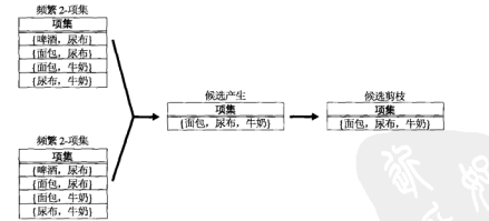
由图可见 $F_{k-1} \times F_{k-1}$ 候选产生过程只产生一个候选 3-项集，这与 $F_{k-1} \times F_{1}$ 方法产生 4 个候选 3-项集相比数量有相当大的减少。

候选项集的剪枝

零候选 k-项集 $X=\{i_1, i_2, \dots, i_k\}$，其 k 个真子集用 $X-\{i_j\} ( \forall j=1,2,\dots,k )$ 表示。按照 Apriori 原理，真子集中有任何一个是非频繁的，$X$ 会被立刻剪枝。需要注意的是，不必明确要求 $X$ 的所有大小不超过 k-1 的子集是频繁的，只需要考虑 k-1。

1. 对于暴力方法生成的候选集，候选剪枝只需要对每个候选 k-项集检查其 k 个长度为 k-1 的子集。
2. 对于 $F_{k-1} \times F_{1}$ 方法，由于保证了每个候选 k-项集至少有 1 个大小为 k-1 的子集是频繁的，所以只需要检查剩余的 k-1 个子集。
3. 对于 $F_{k-1} \times F_{k-1}$ 方法，由于保证了至少有 2 个大小为 k-1 的子集是频繁的，所以只需要对每个候选 k-项集检查其 k-2 个子集。

贡献者

dingyuqi

更新日志

2025/11/8 05:39

查看所有更新日志

• ab415-fix(docs): format issues于 2025/11/8
• 2749d-improve(theme): upgrade于 2025/10/16
• 941fa-feat(theme): upgrade and use collections于 2025/10/11
• eb6eb-improve(docs): use pangu formatter于 2025/8/5
• 86b59-improve(docs): use new table grammar于 2025/8/4
• c9eec-improve(docs): Typesetting于 2025/7/24
• 2185e-improve(docs): use chinese punctuation于 2025/3/6
• fea7c-improve(docs): delete extra whitespace and blank lines于 2025/1/21
• c1c02-modify(docs): remanage folders and rename files于 2024/12/17
• 8b943-docs: update docs于 2024/12/2

版权所有

版权归属：dingyuqi

许可证：署名-非商业性-禁止演绎 4.0 国际 (CC-BY-NC-ND-4.0)

编辑此页