频繁项集的产生 ( 2 )
在 上一节 中我们简单介绍了先验原理以及该算法中的两个关键步骤:候选集的产生和剪枝。
本节将继续介绍支持度的计数以及计算复杂度,这样关于频繁项集的产生的内容就全部介绍完毕。
支持度计数
支持度计数的作用:确定在候选剪枝步骤中保留下来的每个候选项集出现的频繁程度。支持度计数出现在 伪代码 的第 6~11 步实现。
暴力方法
将每个事务与所有的候选项集进行比较,并更新包含在事务中的候选项集的支持度。
这种方法的计算开销十分高,尤其是事务和候选项集的数目都很大时。
枚举方法
枚举每个事务所包含的项集,并利用其更新对应的候选项集的支持度。
例如,考虑事务 ,它包含 5 个项 {1,2,3,5,6}。对于想要考察的候选 3-项集来说,事务 中共有 个 3-项集,其中一定有部分项集是与候选 3-项集重合的,此时增加其支持度,而不对应的子集则可以忽略。
下图给出了一个系统地枚举事务 中所有 3-项集的方法。
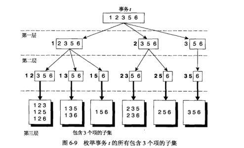
将所有项按照字典顺序排列。
针对于需要生成的 k-项集,选出 k 个最小项,其他较大项跟随在后面。
例如,给定 的 3-项集一定以项 1,2, 3 生成的。 表示的 3-项集是从 1 开始,后随两个取自集合 的项。
下一层的生成重复 2 的动作,但是前缀的数量加一。
Hash 树方法
刚刚提到的枚举方法中我们知道了如何系统地枚举事务所包含的项集。但是如果要进行支持度计数,则还需要将候选项集与生成的 k-项集进行匹配,如果候选项集与枚举出来的项集匹配则支持度加一。那么下面我们将解释如何使用 Hash 树来进行匹配这个动作,这种存储候选集的结构可以大大减少比较的次数。因为不在需要每个事务和每个候选集进行比较,而是每个事务和 Hash 树中特定的候选集进行比较。
我们仍然以书中的例子来看。假设我们已经有了候选 3-项集,一共 15 个。候选集如下:
1. 建立 Hash 树
前置准备
确定 Hash 函数。
例如书中选用的函数: ,这会把与 3 取余之后结果相同的数值分到一个 Hash 分支中。
最大叶子节点数。
如果一个叶子节点中所包含的数据个数超过最大叶子节点数,则说明该叶子节点需要进一步的分裂。此处将该数值设定为 3。
接下来我们需要开始建立这棵树。
详情
对于项集 来说,第一项为 1,根据 Hash 函数,我们应该将其放在左子树上。
同理, 也放在左子树。
我们继续看下一个候选项 。根据第一项 4 可以判断其也应该放在左子树,但是此时左子树的数据数量以及达到最大叶子节点数,所以需要进行分裂。我们根据这三个候选集的第二项进行 Hash 处理,可得到分裂的结果为:
再下一个候选项 的第一项是 1 应该在第一层的左子树,第二项 2 应该在第二层的中间子树。此时第二层的中间子树数据个数又一次超过最大叶子节点数,所以该节点再一次分裂成:
根据以上的规律,不断将候选项加入到树中,我们最终可以得到一棵完整的 Hash 树:
2. 计算出一个事务可能的候选项集
很显然我们在上一节 候选项集的产生 中已经详细介绍过方法。
3. 使用 Hash 树进行计数
我们仍然以事务 为例。
所有 3-项集中候选项的首项为 1 的对左子树进行比较,而首项为 2 的则选择中间子树。首项为 3 的则选择右子树。接下来继续分析项集的第二项,然后根据其数值选择下一层的子树分支。
最后每个候选项必然走到一个叶子节点,其仅仅需要与该节点上的数据进行比较从而计算支持度即可。
计算复杂度
Apriori 算法的计算复杂度受到如下因素的影响。
支持度阈值
降低支持度阈值通常会导致更多的项集被判断为频繁的,这很不利于计算。
项数 ( 维度 )
项数主要影响的是内存的占用情况。而且随着维度的增加,算法产生的候选项更多,时间上也会增加。
事务数
由于 Apriori 算法反复扫描事务数据集,因此运行时间随着事务数的增加而增加。
事务的平均宽度
对于稠密数据集,事务的平均宽度可能很大。
- 频繁项集的最大长度随着事务平均宽度的增加而增加。这会导致候选项产生和支持度计数需要考察更多的项集。
- 随着事务宽度的增加,事务中会包含更多的项集,这将增加支持度计数时 Hash 树遍历的次数。
总结
至此,频繁项集的产生的相关内容就介绍完毕。
