Centrality algorithms are used to understand the influence of specific nodes in a graph and their impact on the network, which can help us identify the most important nodes.

This article will introduce the following algorithms:

• Degree Centrality Algorithm: It can be used as a benchmark indicator of connectivity.
• Closeness Centrality Algorithm: It is used to measure the centrality of a node in a group.
• Betweenness Centrality Algorithm: Used to find control points in a graph.

Degree Centrality

Used to measure the number of relationships a node has. The larger the value, the higher its centrality.

• Input: G = (V, E).
• Output: Each node and its degree centrality value.

Implementation Principle

$$C'_D(N_i) = \frac{N_{degree}}{n - 1}$$

Where:

• $N_{degree}$ represents the degree of the node.
• $n$ represents the number of nodes.

This formula has been standardized.

Adaptation For Heterogeneous Graphs

• This indicator calculation does not involve attributes, only the degree of the graph structure.
• Only the degree under the same label is calculated.

Closeness Centrality

Used to discover nodes that can efficiently propagate information through subgraphs, The higher the value, the shorter the distance between it and other nodes. This algorithm can be used when you need to know which node has the fastest propagation speed.

• Input: G = (V, E).
• Output: Each node and its closeness centrality.

Implementation Principle

The indicator for measuring the centrality of a node is its average distance to other nodes. The closeness centrality algorithm calculates the sum of its distances to other nodes on the basis of calculating the shortest path between all node pairs, and then calculates the inverse of the result.

$$C(u) = \frac{1}{\sum_{v=1}^{n-1}d(u,v)}$$

Where:

• $u$ represents a node.
• $n$ represents the number of nodes in the graph.
• $d(u,v)$ represents the shortest distance between another node $v$ and node $u$.

It is more common to normalize the calculation result to represent the average length of the shortest path, rather than the sum of the shortest paths. The normalization formula is as follows:

$$C_{norm}(u) = \frac{n-1}{\sum_{v=1}^{n-1}d(u,v)}$$

Adaptation For Heterogeneous Graphs

• Only calculate nodes with the same label.
• Actually only calculate the close centrality in each connected subgraph.

Wasserman & Faust algorithm

This algorithm is a variant for non-connected graphs.

$$C_{WF}(u) = \frac{n-1}{N-1}\left(\frac{n-1}{\sum_{v=1}^{n-1}d(u,v)} \right)$$

Where:

• $u$ represents a node.
• $N$ represents the total number of nodes.
• $n$ represents the number of nodes in the same component as $u$.
• $d(u, v)$ represents another node The shortest distance from $v$ to $u$.

Betweenness Centrality

Used to detect the degree of influence of a node on the information flow or resources in the graph, usually used to find nodes that bridge one part of the graph with another.

• Input: G = (V, E).
• Output: Each node and its betweenness centrality value.

Implementation Principle

$$BC(v) = \sum_{s \neq u \neq t} \frac{\sigma_{st}(v)}{\sigma_{st}}$$

Where:

• $v$ represents a node.
• $\sigma_{st}$ represents the sum of the shortest paths between nodes $s$ and $t$.
• $\sigma_{st}(v)$ represents the number of shortest paths between $s$ and $t$ that pass through node $v$.

In simple terms, betweenness centrality measures the node $v$ by the proportion of the shortest paths between point pairs that pass through node $v$. Importance.

The following figure shows the steps to calculate the betweenness score.

Betweenness centrality calculation example

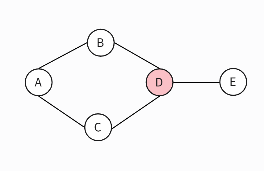
The calculation process for node D is as follows:

Shortest path node pairs through D	Total number of shortest paths between node pairs $p$	Percentage of the number of shortest paths through D $\frac{p(u)}{p}$
(A, E)	1	1
(B, E)	1	1
(C, E)	1	1
(B, C)	2 (B->A->C and B->D->C respectively)	0.5

So according to the formula, the betweenness score of node D is: 1 + 1 + 1 + 0.3 = 3.5.

Algorithm Steps

Different from linear sequential programming calculations, the algorithm given here is based on Pregel's message propagation method for calculation. It is only for reference.

Step 1: Calculate the shortest path and the number of shortest paths between all pairs of points

1. Initialization
   • For source node $s$, path count $\sigma_s = 1$, path length $d_s = 0$.
   • For other nodes, path count $\sigma = 0$, path length $d = \infty$.
2. Message propagation Assume that node $u$ sends a message to node $v$.
   • Node $u$ message sends: $(d_u +1, \sigma_u)$, that is, path length and number of paths.
   • Node $v$ message update:
   • If $d_{new} < d_{current}$: update the shortest path length $d_v = d_{new}$, set the number of paths $\sigma_v=\sigma_u$.
   • If $d_{new} = d_{current}$: It means that another path of equal length has been found, so the number of paths is increased by $\sigma_v += \sigma_u$.

Step 2: Calculate the contribution value of each point

$$contribution = \frac{\sigma_{sv} \times \sigma_{vt}}{\sigma_{st}}$$

Suppose we have three nodes: source node $s$, intermediate node $v$ and target node $t$. What we need to calculate is: the proportion of the path passing through node $v$ to all shortest paths from $s$ to $t$. The $\sigma_{sv} \times \sigma_{vt}$ in the formula is the number of shortest paths between $s$ and $t$ that pass through $v$, which is the combination principle of the shortest path from $s$ to $t$. The shortest path of $t$ is considered as the combination of the path from $s$ to $v$ and the path from $v$ to $t$.

betweenness_centrality.py

def calculate_betweenness_centrality(source, all_nodes):
    BC_s = 0

    for t in all_nodes:
        if t == source:
            continue

        for v in all_nodes:
            if v == source or v == t:
                continue
            sigma_sv = get_shortest_path_count(source, v)
            sigma_vt = get_shortest_path_count(v, t)
            sigma_st = get_shortest_path_count(source, t)

            if sigma_st == 0:
                continue

            contribution = (sigma_sv * sigma_vt) / sigma_st

            BC_s += contribution

    return BC_s

Adaptation For Heterogeneous Graphs

• This indicator calculation does not involve attributes, only the degree of the graph structure.
• Only calculate the degree under the same label.

Summary

This article introduces three different centrality algorithms, each of which identifies important nodes in the graph from different perspectives.

• Degree centrality algorithm

  The importance of nodes is evaluated by calculating the in-and-out degree of each node. Nodes with high degree centrality mean that they are connected to more nodes.

• Closeness centrality

  The importance of nodes is measured by calculating the average distance to other nodes. Nodes with high closeness centrality mean a more central position in the graph, and the path from it to all other nodes is shorter, which will be faster if messages are propagated.

• Betweenness centrality

  The importance of nodes is measured by calculating the probability that the shortest path between other nodes passes through itself. It is usually used to detect the degree of influence of nodes on information flow or resources in the graph. Nodes with high betweenness centrality mean that they are important bridges between two groups of nodes in the graph.

References for this article

1. "Graph Algorithms for Data Analysis: Based on Spark and Neo4j"

Contributors

• dingyuqi

Changelog

Last Updated: View All Changelog

• 42218-

  fix(docs): text typo

  On 1/22/25
• 1289a-

  improve(docs): delete extra whitespace and blank lines

  On 1/21/25
• fdfc7-

  improve(docs): add summary

  On 1/9/25
• 13feb-

  fix(docs): fix text typo

  On 12/30/24
• dc65c-

  fix(docs): optimize articles

  On 12/27/24
• d8792-

  feat(docs): add new english articles

  On 12/18/24

Copyright

Copyright Ownership:dingyuqi

This article link:/en/article/centrality-algorithms/

License under:Attribution-NonCommercial-NoDerivatives 4.0 International (CC-BY-NC-ND-4.0)